Simulate Coupled Dipoles

Note: See the background section on Coupled Lorentz oscillators or the PyCharge paper for more information about the underlying physics of coupled dipoles.

Two coupled dipoles modeled as Lorentz oscillators (LOs) in a system can be simulated in PyCharge, and their modified radiative properties can be calculated. An example program code for simulating two s dipoles (transverse), which are polarized along the \(y\) axis and separated by 80 nm along the \(x\) axis, is shown below:

import pycharge as pc
from numpy import pi
timesteps = 40000
dt = 1e-18
omega_0 = 100e12*2*pi
origins = ((0, 0, 0), (80e-9, 0, 0))
init_r = (0, 1e-9, 0)
sources = (pc.Dipole(omega_0, origins[0], init_r),
           pc.Dipole(omega_0, origins[1], init_r))
simulation = pc.Simulation(sources)
simulation.run(timesteps, dt, 's_dipoles.dat')
d_12, g_plus = pc.calculate_dipole_properties(
    sources[0], first_index=10000)
d_12_th, g_12_th = pc.s_dipole_theory(
    r=1e-9, d_12=80e-9, omega_0=omega_0)

The two dipoles have a natural angular frequency \(\omega_0\) of \(200\pi\times10^{12}\) rad/s and are simulated over 40,000 time steps (with a time step \(dt\) of \(10^{-18}\) s). The two charges in the dipole both have a mass of \(m_e\) (the effective mass of the dipole is \(m_e/2\)) and a charge magnitude of \(e\). Once the simulation is complete, the Simuation and related source objects are saved into the file s_dipoles.dat, which can be accessed for analyses. The dipoles begin oscillating in phase with an initial charge displacement \(\mathbf{r}_{\mathrm{dip}}\) of 1 nm, resulting in superradiance and a modified SE rate \(\gamma^+\). The rate \(\gamma^+\) and frequency shift \(\delta_{12}\) are then calculated in PyCharge by curve fitting the kinetic energy of the dipole (using the kinetic energy values after the 10,000 time step). As well, the theoretical values for \(\gamma_{12}\) and \(\delta_{12}\) are calculated by PyCharge.

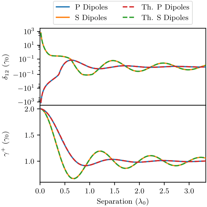
The radiative properties of two coupled dipoles as a function of separation can be calculated by repeatedly running the previous simulation while sweeping across a range of dipole separation values. Using this technique, the modified rate \(\gamma^+\) and frequency shift \(\delta_{12}\) for in phase (superradiant) s and p dipoles, scaled by the free-space emission rate \(\gamma_0\), are plotted below. The theoretical results from QED theory are also shown, and the Python script can be found at examples/paper_figures/figure7:

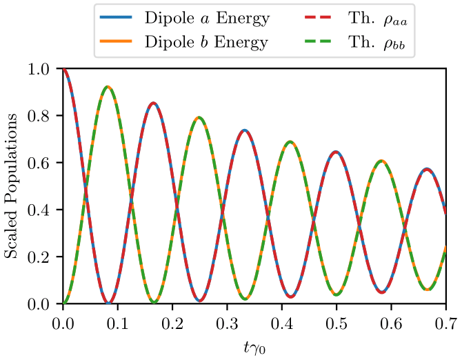
We can also plot the normalized populations of the excited states of two coupled dipoles, \(\rho_{aa}(t)\) and \(\rho_{bb}(t)\), using the normalized total energy of the dipoles at each time step. This yields particularly interesting results for coupled dipoles with small separations when one dipole is initially excited (\(\rho_{aa}(0)=1\)) and the other is not (\(\rho_{bb}(0)=0\)). In this scenario, the populations are a linear combination of the superradiant and subraddiant states, which leads to the observed energy transfer between dipoles known as Förster coupling. This phenomenon can be simulated in PyCharge by initializing the excited dipole with a much larger dipole moment (and total energy) than the other. The simulation results and analytical solution are shown below, and the script is given at examples/paper_figures/figure8:

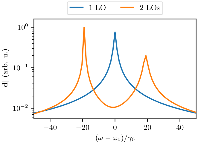
Additionally, the dipole moment of one of the dipoles in the frequency domain is shown below, which clearly shows the frequency peaks of the subradiant and supperradiant states. The dipole moment of an isolated LO in the frequency domain is also shown for comparison, and the Python script can be found at examples/paper_figures/figure9: