Dipole Simulation

In the last section, we calculated the fields and potentials in 3D space generated by an oscillating point charge at a specified time. This required using the OscillatingCharge class, which has a predefined trajectory. However, PyCharge can also simulate dipoles that act as Lorentz oscillators, where the trajectories of the charges in the dipole are not predefined. These are simulated in PyCharge using the Dipole class.

The two opposite (positive and negative) charges in the Dipole object do not have predefined trajectories, since the dipole's moment is dependent on the external electric field that acts as a driving force. The dipole moment is defined by the driven oscillator differential equation, which is solved dynamically in PyCharge at each time step. For more information about Dipole objects and how they are simulated in PyCharge, see the Lorentz Oscillators section.

Here, we provide a script (found at examples/s_dipoles.py) for simulating two transverse dipoles (s-dipoles) that act as Lorentz oscillators. We run the simulation over 40,000 time steps and then analyze the dipole moment as a function of time to determine the new decay rate (\(\gamma\)) and frequency shift (\(\delta_{12}\)). We then compare these results to the theoretical Green's function values.

First, we import the necessary Python packages and define the simulation variables. The two dipoles are separated by 80 nm along the \(x\)-axis and are both polarized in the \(y\) direction with an initial charge separation of 1 nm. Each point charge is instantiated with the default values for the charge (e) and mass (m_e). Note that the effective mass of the dipole is m_e/2, as discussed in the Lorentz Oscillators section. The simulation is run over 40,000 time steps and uses a time step of 1e-18:

import numpy as np
import pycharge as pc

# Simulation variables
init_r = 1e-9  # Initial charge separation along y-axis
d_12 = 80e-9  # Distance between dipoles along x-axis
omega_0 = 100e12*2*np.pi  # Natural angular frequency of the dipoles
timesteps = 40000  # Number of time steps in the simulation
dt = 1e-18  # Time step

origin_list = ((0, 0, 0), (d_12, 0, 0))  # Dipole origin vectors
init_r_list = ((0, init_r, 0), (0, init_r, 0))  # Initial charge displacements
sources = (pc.Dipole(omega_0, origin_list[0], init_r_list[0]),
           pc.Dipole(omega_0, origin_list[1], init_r_list[1]))
simulation = pc.Simulation(sources)

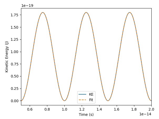
Next, we run the simulation. The dipole moment, as well as the electric driving fields, are saved to the Dipole object at each time step. When the simulation is completed, the Simulation object (which includes the Dipole objects) is saved to the file s_dipoles.dat. We then compute the theoretical decay rate and frequency shift of the dipoles from the Green's function using the s_dipole_theory method. Finally, we calculate these properties from the kinetic energy of the dipole using the calculate_dipole_properties method, which also plots the actual kinetic energy and the estimated function fit:

# Simulation data of dipoles is saved to file 's_dipoles.dat'
simulation.run(timesteps, dt, 's_dipoles.dat')

# Calculate theoretical \delta and \gamma_12
theory_delta_12, theory_gamma_12 = pc.s_dipole_theory(init_r, d_12, omega_0)
# Calculate \delta and \gamma from simulation starting from 5000 time steps
delta_12, gamma = pc.calculate_dipole_properties(
    sources[0], first_index=10000, plot=True
)
print('Delta_12 (theory):', theory_delta_12)
print('Delta_12 (simulation):', delta_12)
print('Gamma_12 (theory):', theory_gamma_12)
print('Gamma (simulation):', gamma)
print()

The output plot and values are shown below. Note that since the dipoles started in-phase, the decay rate values are related by \(\gamma=1+\gamma_{12}\).

Delta_12 (theory): 156.92644882498607
Delta_12 (simulation): 156.9188149970173
Gamma_12 (theory): 0.9943859767792077
Gamma (simulation): 1.9970287120394974