Stationary Charge Fields

Here we present a simulation script, found in examples/stationary_charge.py, that uses PyCharge to calculate the components of the electric field \((E_x, E_y, E_z)\) generated by a stationary charge located at the origin position \((0, 0, 0)\). The electric field components are plotted along the \(x\)-\(y\) plane on a symmetrical logarithmic scale to account for both positive and negative values.

First we import the required packages:

import matplotlib as mpl
import matplotlib.pyplot as plt
import numpy as np
from mpl_toolkits.axes_grid1.inset_locator import inset_axes

import pycharge as pc

Point charges are represented in PyCharge using subclasses from the parent class Charge. These objects define the trajectories (position, velocity, and acceleration) of the charges in \(x\), \(y\), and \(z\). Here, we use the class StationaryCharge which is instantiated with the default charge value e and a position vector. The fields and potentials generated by the point charges at a specified time are calculated using the Simulation class. The electric field is calculated by the Simulation object using the calculate_E method, which requires the time of simulation and the meshgrid of points being calculated in \(x\), \(y\), and \(z\):

# Create charge and simulation objects
source = pc.StationaryCharge(position=(0, 0, 0))
simulation = pc.Simulation(source)

# Create meshgrid in x-y plane between -10 nm to 10 nm at z=0
lim = 10e-9
npoints = 1000  # Number of grid points
coordinates = np.linspace(-lim, lim, npoints)  # grid from -lim to lim
x, y, z = np.meshgrid(coordinates, coordinates, 0, indexing='ij')  # z=0

# Calculate E field components at t=0
E_x, E_y, E_z = simulation.calculate_E(t=0, x=x, y=y, z=z)

Now that we have calculated the components of the \(\mathbf{E}\) field, we can plot them using matplotlib. The values of the field components are stored as 3D numpy arrays, with indices corresponding to the meshgrid position values. Finally, the three field components are plotted with a corresponing colorbar:

# Plot E_x, E_y, and E_z fields
E_x_plane = E_x[:, :, 0]  # Create 2D array at z=0 for plotting
E_y_plane = E_y[:, :, 0]
E_z_plane = E_z[:, :, 0]

# Create figs and axes, plot E components on log scale
fig, axs = plt.subplots(1, 3, sharey=True)
norm = mpl.colors.SymLogNorm(linthresh=1.01e6, linscale=1, vmin=-1e9, vmax=1e9)
extent = [-lim, lim, -lim, lim]
im_0 = axs[0].imshow(E_x_plane.T, origin='lower', norm=norm, extent=extent)
im_1 = axs[1].imshow(E_y_plane.T, origin='lower', norm=norm, extent=extent)
im_2 = axs[2].imshow(E_z_plane.T, origin='lower', norm=norm, extent=extent)

# Add labels
for ax in axs:
    ax.set_xlabel('x (nm)')
axs[0].set_ylabel('y (nm)')
axs[0].set_title('E_x (N/C)')
axs[1].set_title('E_y (N/C)')
axs[2].set_title('E_z (N/C)')

# Add colorbar to figure
Ecax = inset_axes(
    axs[2], width="6%", height="100%", loc='lower left',
    bbox_to_anchor=(1.05, 0., 1, 1), bbox_transform=axs[2].transAxes, borderpad=0
)
E_cbar = plt.colorbar(im_2, cax=Ecax)  # right of im_2
E_cbar.ax.set_ylabel('E (N/C)', rotation=270, labelpad=12)

plt.show()

The output plot is shown below:

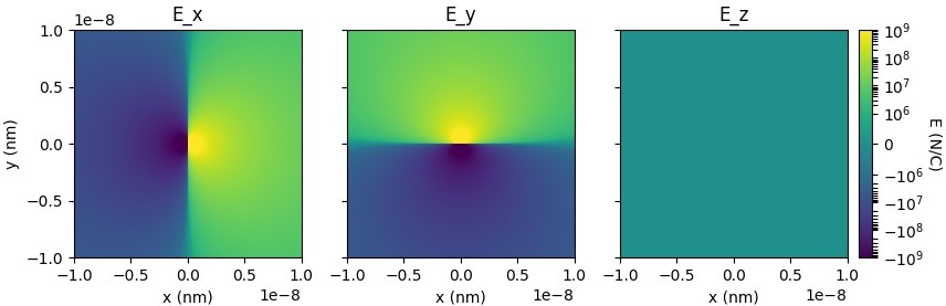
As expected, the \(E_z\) field is zero because we are plotting along the \(x\)-\(y\) plane.