Oscillating Charge Fields

In the last section we presented a simulation script for calculating the electric field generated by a stationary point charge. Here, we will calculate the fields and potentials generated by an oscillating point charge. The charge is oscillating sinusoidally along the \(x\)-axis with an amplitude of 0.1 nm and an angular frequency \(\omega=5\times10^{17}\) rad/s. To calculate the components of the electric field (\(E_x\), \(E_y\), \(E_z\)) generated by the oscillating point charge at time \(t=0\) s, we can reuse the Python script from the previous section and instantiate an OscillatingCharge object instead of a StationaryCharge object:

charge = pc.OscillatingCharge(origin=(0, 0, 0), direction=(1, 0, 0),
                              amplitude=1e-10, omega=5e17)

That's it! The output plot is shown below:

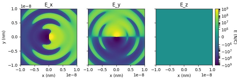
Once again, as expected, the \(E_z\) field is zero because we are plotting along the \(x\)-\(y\) plane and the charge is oscillating along the \(x\)-axis.

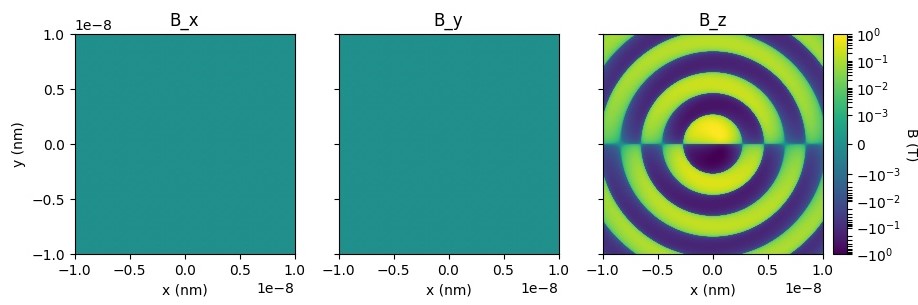
Next, we can calculate the \(\mathbf{B}\) field by replacing the method simulation.calculate_E with simulation.calculate_B, as well as changing some plot labels throughout the script:

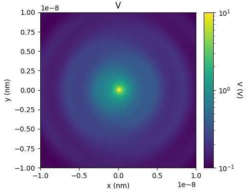
Finally, we can plot the scalar (\(\Phi\) or \(V\)) and vector potentials (\(\mathbf{A}\)) using the simulate.calculate_V and simulate.calculate_A methods:

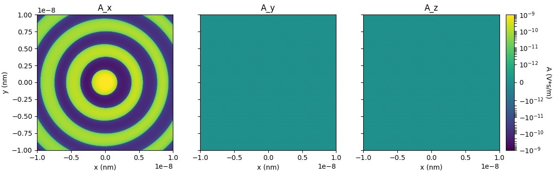
The full script for plotting all of the above figures can be found at examples/oscillating_charge.py.