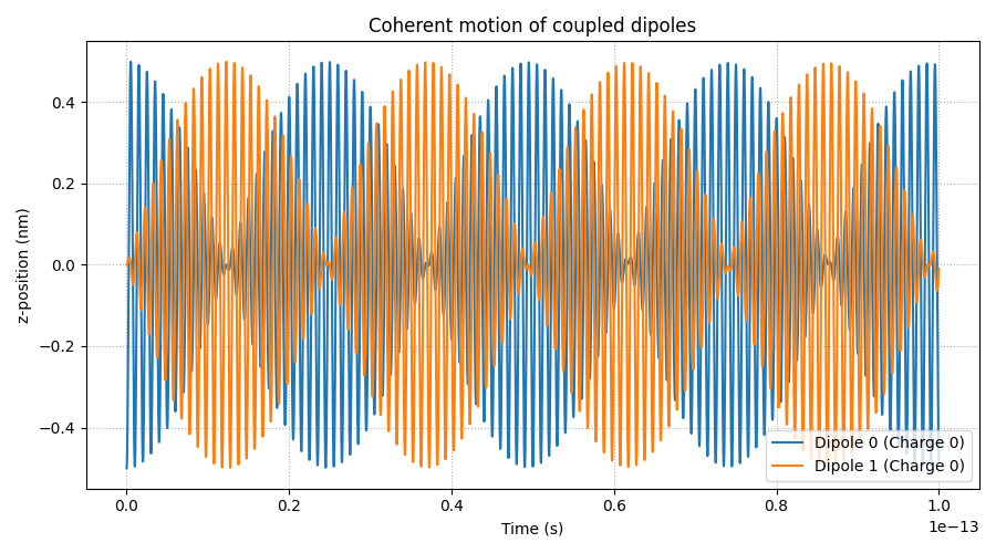
Simulate Coupled Dipoles

This example demonstrates the coherent oscillations between two nearby Lorentz oscillators (dipoles). When placed in close proximity, the dipoles interact through their electromagnetic fields, leading to synchronized motion. One dipole is initialized in an excited state, while the other starts in its ground state.

Import necessary libraries

import jax
import jax.numpy as jnp
import matplotlib.pyplot as plt
from scipy.constants import e, m_e

from pycharge import dipole_source, simulate

jax.config.update("jax_enable_x64", True)

Define dipoles and simulation timeline

initial_moment0 = [0.0, 0.0, 1e-9]  # Initial excited state along z-axis
initial_moment1 = [0.0, 0.0, -1e-20]  # Initial ground state along -z-axis
q = e * 20  # Charge magnitude for each dipole
omega_0 = 1e15 * 2 * jnp.pi  # 1 PHz natural frequency
m = m_e  # Electron mass
origin0 = [0.0, 0.0, 0.0]  # Origin of first dipole
origin1 = [0.0, 5e-9, 0.0]  # Origin of second dipole (5 nm apart)

# Create two identical dipoles separated along the y-axis
dipole0 = dipole_source(initial_moment0, omega_0, origin0, q, m)
dipole1 = dipole_source(initial_moment1, omega_0, origin1, q, m)

# Simulation time parameters
num_steps = 10_000
dt = 1e-17  # 10 attoseconds per step
ts = jnp.arange(num_steps) * dt

Run the simulation

sim_fn = jax.jit(simulate([dipole0, dipole1], ts))
states = sim_fn()

Timestep 0
Timestep 100
Timestep 200
Timestep 300
Timestep 400
Timestep 500
Timestep 600
Timestep 700
Timestep 800
Timestep 900
Timestep 1000
Timestep 1100
Timestep 1200
Timestep 1300
Timestep 1400
Timestep 1500
Timestep 1600
Timestep 1700
Timestep 1800
Timestep 1900
Timestep 2000
Timestep 2100
Timestep 2200
Timestep 2300
Timestep 2400
Timestep 2500
Timestep 2600
Timestep 2700
Timestep 2800
Timestep 2900
Timestep 3000
Timestep 3100
Timestep 3200
Timestep 3300
Timestep 3400
Timestep 3500
Timestep 3600
Timestep 3700
Timestep 3800
Timestep 3900
Timestep 4000
Timestep 4100
Timestep 4200
Timestep 4300
Timestep 4400
Timestep 4500
Timestep 4600
Timestep 4700
Timestep 4800
Timestep 4900
Timestep 5000
Timestep 5100
Timestep 5200
Timestep 5300
Timestep 5400
Timestep 5500
Timestep 5600
Timestep 5700
Timestep 5800
Timestep 5900
Timestep 6000
Timestep 6100
Timestep 6200
Timestep 6300
Timestep 6400
Timestep 6500
Timestep 6600
Timestep 6700
Timestep 6800
Timestep 6900
Timestep 7000
Timestep 7100
Timestep 7200
Timestep 7300
Timestep 7400
Timestep 7500
Timestep 7600
Timestep 7700
Timestep 7800
Timestep 7900
Timestep 8000
Timestep 8100
Timestep 8200
Timestep 8300
Timestep 8400
Timestep 8500
Timestep 8600
Timestep 8700
Timestep 8800
Timestep 8900
Timestep 9000
Timestep 9100
Timestep 9200
Timestep 9300
Timestep 9400
Timestep 9500
Timestep 9600
Timestep 9700
Timestep 9800
Timestep 9900

Plot the trajectory of one charge from each dipole

z_dipole0 = jnp.asarray(states[0][:, 0, 0, 2])
z_dipole1 = jnp.asarray(states[1][:, 0, 0, 2])

plt.figure(figsize=(9, 5))
plt.plot(ts, z_dipole0 * 1e9, label="Dipole 0 (Charge 0)")
plt.plot(ts, z_dipole1 * 1e9, label="Dipole 1 (Charge 0)")
plt.xlabel("Time (s)")
plt.ylabel("z-position (nm)")
plt.title("Coherent motion of coupled dipoles")
plt.legend()
plt.grid(True, which="both", ls=":")
plt.tight_layout()
plt.show()