Current Coil Magnetic Field

This example visualizes the magnetic field produced by a current coil and compares it with the analytical Biot-Savart law solution. We model the coil using discrete charges moving in a circular trajectory and calculate the z-component of the magnetic field along the central axis.

Import necessary libraries

import jax
import jax.numpy as jnp
import matplotlib.pyplot as plt
from matplotlib import colors
from scipy.constants import e, mu_0

from pycharge import Charge, potentials_and_fields

jax.config.update("jax_enable_x64", True)

Define the current coil

A current coil is modeled as discrete charges moving in a circular trajectory with constant angular velocity. Each charge is placed at a different phase angle.

num_charges = 30  # Number of discrete charges in the ring
R = 1e-2  # Coil radius (1 cm)
omega = 1e8  # Angular velocity (rad/s)


def get_circular_position(phi):
    """Returns a function for a circular trajectory with a given phase."""

    def position(t):
        x = R * jnp.cos(omega * t + phi)
        y = R * jnp.sin(omega * t + phi)
        z = 0
        return [x, y, z]

    return position


charges = [
    Charge(position_fn=get_circular_position(phi), q=e)
    for phi in jnp.linspace(0, 2 * jnp.pi, num_charges, endpoint=False)
]

Set up the observation grid

Create a 2D grid in the x-y plane to visualize the magnetic field.

grid_res = 500
grid_extent = 1.5 * R

x = jnp.linspace(-grid_extent, grid_extent, grid_res)
y = jnp.linspace(-grid_extent, grid_extent, grid_res)
z = jnp.array([0.0])
t = jnp.array([0.0])

X, Y, Z, T = jnp.meshgrid(x, y, z, t, indexing="ij")

Calculate electromagnetic quantities

Compute all potentials and fields at once using a JIT-compiled function.

calculate_fields = jax.jit(potentials_and_fields(charges))
result = calculate_fields(X, Y, Z, T)

# Extract z-component of magnetic field
magnetic_field_z = result.magnetic.squeeze()[:, :, 2]

extent = (float(x[0]), float(x[-1]), float(y[0]), float(y[-1]))

Plotting utilities

def _sym_log_norm(data):
    """Symmetric logarithmic normalization."""
    vmax = float(jnp.max(jnp.abs(data)))
    return None if vmax == 0 else colors.SymLogNorm(linthresh=vmax * 1e-5, linscale=1, vmin=-vmax, vmax=vmax)


def _setup_axis(ax, title, xlabel="x (m)", ylabel="y (m)"):
    """Configure axis with labels and title."""
    ax.set_xlabel(xlabel)
    ax.set_ylabel(ylabel)
    ax.set_title(title)


def plot_field_2d(data, title, cbar_label, cmap="RdBu_r", norm=None):
    """Plot a 2D scalar field."""
    fig, ax = plt.subplots(figsize=(8, 6))
    norm = norm or _sym_log_norm(data)
    im = ax.imshow(data.T, origin="lower", cmap=cmap, norm=norm, extent=extent)
    fig.colorbar(im, ax=ax, label=cbar_label)
    _setup_axis(ax, title)
    fig.tight_layout()
    plt.show()

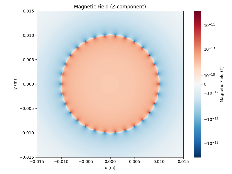
Magnetic field (z-component)

The z-component of the magnetic field \(B_z\) is strongest at the center of the coil and decreases with distance. The field is perpendicular to the plane of the coil.

plot_field_2d(
    magnetic_field_z,
    title="Magnetic Field (Z-component)",
    cbar_label="Magnetic Field (T)",
    cmap="RdBu_r",
)

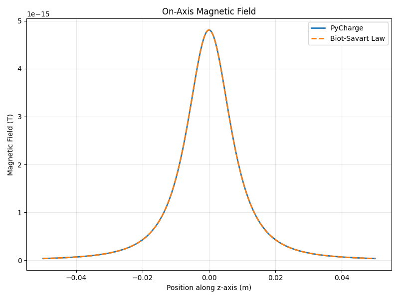
Comparison with Biot-Savart law

We compare the magnetic field along the z-axis with the analytical solution. The Biot-Savart law gives \(B_z = \frac{\mu_0 I R^2}{2(z^2 + R^2)^{3/2}}\) for the on-axis field of a current loop.

z_axis = jnp.linspace(-5 * R, 5 * R, 500)
x_axis = jnp.zeros_like(z_axis)
y_axis = jnp.zeros_like(z_axis)
t_axis = jnp.zeros_like(z_axis)

result_1d = calculate_fields(x_axis, y_axis, z_axis, t_axis)
B_pycharge = result_1d.magnetic[:, 2]

current = num_charges * e * omega / (2 * jnp.pi)
B_biot_savart = mu_0 * current * R**2 / (2 * (z_axis**2 + R**2) ** (3 / 2))

fig, ax = plt.subplots(figsize=(8, 6))
ax.plot(z_axis, B_pycharge, label="PyCharge", linewidth=2)
ax.plot(z_axis, B_biot_savart, "--", label="Biot-Savart Law", linewidth=2)
ax.set_xlabel("Position along z-axis (m)")
ax.set_ylabel("Magnetic Field (T)")
ax.set_title("On-Axis Magnetic Field")
ax.legend()
ax.grid(True, alpha=0.3)
fig.tight_layout()
plt.show()