Oscillating Dipole Fields

This example visualizes the electromagnetic potentials and fields produced by an oscillating electric dipole. The dipole consists of two opposite charges that oscillate harmonically along the y-axis. We calculate and plot the scalar potential, vector potential, electric field, and magnetic field in the x-y plane at a fixed time.

Import necessary libraries

import jax
import jax.numpy as jnp
import matplotlib.pyplot as plt
import numpy as np
from matplotlib import colors
from scipy.constants import e

from pycharge import Charge, potentials_and_fields

jax.config.update("jax_enable_x64", True)

Define the oscillating dipole

An oscillating dipole consists of two charges with equal magnitude but opposite sign, oscillating harmonically along the y-axis. The charges move with the same amplitude but in opposite directions.

amplitude = 1e-10  # 2 nanometers
omega = 2e18  # Angular frequency (rad/s)
charge_magnitude = e  # Elementary charge (1.6e-19 C)


def positive_charge_position(t):
    """Position of the positive charge oscillating along y-axis."""
    return (0.0, amplitude * jnp.cos(omega * t), 0.0)


def negative_charge_position(t):
    """Position of the negative charge oscillating along y-axis."""
    return (0.0, -amplitude * jnp.cos(omega * t), 0.0)


charges = [
    Charge(position_fn=positive_charge_position, q=charge_magnitude),
    Charge(position_fn=negative_charge_position, q=-charge_magnitude),
]

print(f"Max velocity of charges: {amplitude * omega:.2e} m/s")

Max velocity of charges: 2.00e+08 m/s

Set up the observation grid

Create a 2D grid in the x-y plane to visualize the fields at a specific time.

grid_res = 300
grid_extent = 1e-9  # ±1 nm

x = jnp.linspace(-grid_extent, grid_extent, grid_res)
y = jnp.linspace(-grid_extent, grid_extent, grid_res)
z = jnp.array([0.0])
t = jnp.array([0.0])  # Snapshot at t=0 (maximum separation)

X, Y, Z, T = jnp.meshgrid(x, y, z, t, indexing="ij")

Calculate electromagnetic quantities

Compute all potentials and fields at once using a JIT-compiled function.

calculate_fields = jax.jit(potentials_and_fields(charges))
result = calculate_fields(X, Y, Z, T)

# Extract field components
scalar_potential = result.scalar.squeeze()
electric_field = result.electric.squeeze()
vector_potential = result.vector.squeeze()
magnetic_field = result.magnetic.squeeze()

extent = (float(x[0]), float(x[-1]), float(y[0]), float(y[-1]))

Plotting utilities

def _sym_log_norm(data):
    """Symmetric logarithmic normalization."""
    vmax = float(jnp.max(jnp.abs(data)))
    return None if vmax == 0 else colors.SymLogNorm(linthresh=vmax * 1e-5, linscale=1, vmin=-vmax, vmax=vmax)


def _setup_axis(ax, title, xlabel="x (m)", ylabel="y (m)", grid_color="gray"):
    """Configure axis with labels, title, and grid lines."""
    ax.set_xlabel(xlabel)
    ax.set_ylabel(ylabel)
    ax.set_title(title)


def plot_field_2d(data, title, cbar_label, cmap="RdBu_r", norm=None):
    """Plot a 2D scalar field."""
    fig, ax = plt.subplots(figsize=(8, 6))
    norm = norm or _sym_log_norm(data)
    im = ax.imshow(data.T, origin="lower", cmap=cmap, norm=norm, extent=extent)
    fig.colorbar(im, ax=ax, label=cbar_label)
    _setup_axis(ax, title, grid_color="gray" if cmap == "RdBu_r" else "white")
    fig.tight_layout()
    plt.show()


def plot_vector_components(vector_data, title_prefix, cbar_label_prefix):
    """Plot x, y, z components of a vector field."""
    fig, axes = plt.subplots(1, 3, figsize=(15, 4))

    for idx, (ax, comp) in enumerate(zip(axes, ["x", "y", "z"])):
        data = vector_data[:, :, idx].T
        im = ax.imshow(data, origin="lower", cmap="RdBu_r", norm=_sym_log_norm(data), extent=extent)
        fig.colorbar(im, ax=ax, label=f"${cbar_label_prefix}_{{{comp}}}$")
        _setup_axis(ax, f"{title_prefix}: {comp.upper()}-component")

    fig.tight_layout()
    plt.show()


def plot_field(vector_field, title, cbar_label, streamlines=False, skip=10):
    """Plot field magnitude with optional streamlines."""
    magnitude = jnp.linalg.norm(vector_field, axis=-1)

    # Downsample for streamlines
    X_stream = np.array(X[::skip, ::skip, :, :].squeeze())
    Y_stream = np.array(Y[::skip, ::skip, :, :].squeeze())
    Fx_stream = np.array(vector_field[::skip, ::skip, 0])
    Fy_stream = np.array(vector_field[::skip, ::skip, 1])

    fig, ax = plt.subplots(figsize=(8, 6))

    # Background: magnitude
    vmin = float(jnp.min(magnitude[magnitude > 0])) if jnp.any(magnitude > 0) else 1e-30
    im = ax.imshow(
        magnitude.T,
        origin="lower",
        cmap="viridis",
        norm=colors.LogNorm(vmin=vmin),
        extent=extent,
    )

    # Foreground: streamlines (only if requested and field is non-zero)
    if streamlines and jnp.max(jnp.abs(vector_field)) > 0:
        ax.streamplot(
            X_stream.T,
            Y_stream.T,
            Fx_stream.T,
            Fy_stream.T,
            color="black",
            density=1.5,
            linewidth=0.8,
            arrowsize=1.0,
        )

    fig.colorbar(im, ax=ax, label=cbar_label)
    _setup_axis(ax, title, grid_color="white")
    ax.set_xlim(extent[0], extent[1])
    ax.set_ylim(extent[2], extent[3])
    fig.tight_layout()
    plt.show()

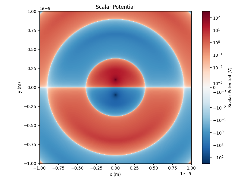
Scalar potential

The scalar potential \(\phi\) exhibits the characteristic dipole pattern. For an oscillating dipole, the potential varies in time and the field pattern propagates outward as electromagnetic radiation.

plot_field_2d(scalar_potential, title="Scalar Potential", cbar_label="Scalar Potential (V)", cmap="RdBu_r")

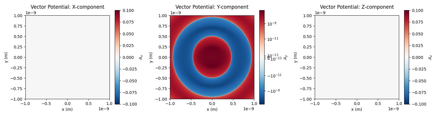
Vector potential

The vector potential \(\mathbf{A}\) is proportional to charge velocity. For oscillating charges with \(\mathbf{v} \neq 0\), the Liénard-Wiechert formulation gives non-zero \(\mathbf{A}\), primarily oriented along the direction of charge motion (y-axis).

plot_vector_components(vector_potential, title_prefix="Vector Potential", cbar_label_prefix="A")

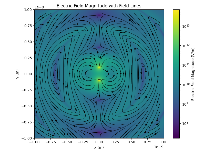
Electric field

The electric field \(\mathbf{E} = -\nabla \phi - \partial \mathbf{A}/\partial t\) can be decomposed into x, y, and z components.

plot_vector_components(electric_field, title_prefix="Electric Field", cbar_label_prefix="E")

The field magnitude shows the dipole pattern and radiation field, with streamlines emerging from the positive charge and terminating at the negative charge.

plot_field(
    electric_field,
    title="Electric Field Magnitude with Field Lines",
    cbar_label="Electric Field Magnitude (V/m)",
    streamlines=True,
)

Magnetic field components

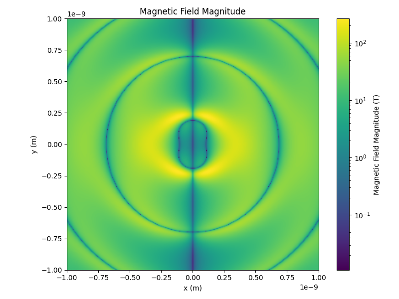
The magnetic field \(\mathbf{B} = \nabla \times \mathbf{A}\) is generated by the oscillating charges. Moving charges create currents, producing a non-zero magnetic field.

plot_vector_components(magnetic_field, title_prefix="Magnetic Field", cbar_label_prefix="B")

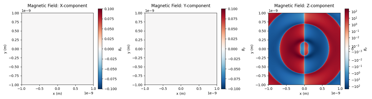
The magnetic field circulates around the dipole axis, perpendicular to both the electric field and direction of propagation.

plot_field(
    magnetic_field,
    title="Magnetic Field Magnitude",
    cbar_label="Magnetic Field Magnitude (T)",
)