Poynting Vector

This example visualizes the Poynting vector for an oscillating electric dipole. The Poynting vector \(\mathbf{S} = \frac{1}{\mu_0} \mathbf{E} \times \mathbf{B}\) represents the directional energy flux of the electromagnetic field.

Import necessary libraries

import jax
import jax.numpy as jnp
import matplotlib.pyplot as plt
from scipy.constants import c, e, mu_0

from pycharge import Charge, potentials_and_fields

jax.config.update("jax_enable_x64", True)

Define the oscillating dipole

An oscillating dipole consists of two charges with equal magnitude but opposite sign, oscillating harmonically along the x-axis.

amplitude = 5e-11  # 50 picometers
omega = (0.8 * c) / amplitude  # Angular frequency (80% speed of light at max velocity)
charge_magnitude = e  # Elementary charge (1.6e-19 C)


def positive_charge_position(t):
    """Position of the positive charge oscillating along x-axis."""
    return (amplitude * jnp.sin(omega * t), 0.0, 0.0)


def negative_charge_position(t):
    """Position of the negative charge oscillating along x-axis."""
    return (-amplitude * jnp.sin(omega * t), 0.0, 0.0)


charges = [
    Charge(position_fn=positive_charge_position, q=charge_magnitude),
    Charge(position_fn=negative_charge_position, q=-charge_magnitude),
]

Set up the observation grid

Create a 2D grid in the x-y plane to visualize the Poynting vector.

grid_res = 800
grid_extent = 1e-9  # ±1 nm

x = jnp.linspace(-grid_extent, grid_extent, grid_res)
y = jnp.linspace(-grid_extent, grid_extent, grid_res)
z = jnp.array([0.0])
t = jnp.array([0.0])  # Snapshot at t=0

X, Y, Z, T = jnp.meshgrid(x, y, z, t, indexing="ij")

Calculate electromagnetic quantities

Compute all potentials and fields at once using a JIT-compiled function.

calculate_fields = jax.jit(potentials_and_fields(charges))
result = calculate_fields(X, Y, Z, T)

# Extract field components
electric_field = result.electric.squeeze()
magnetic_field = result.magnetic.squeeze()

extent = (float(x[0]), float(x[-1]), float(y[0]), float(y[-1]))

Calculate Poynting vector

The Poynting vector \(\mathbf{S} = \frac{1}{\mu_0} \mathbf{E} \times \mathbf{B}\) describes the directional energy flux density of the electromagnetic field.

poynting_vector = jnp.cross(electric_field, magnetic_field, axis=-1) / mu_0
poynting_magnitude = jnp.linalg.norm(poynting_vector, axis=-1)

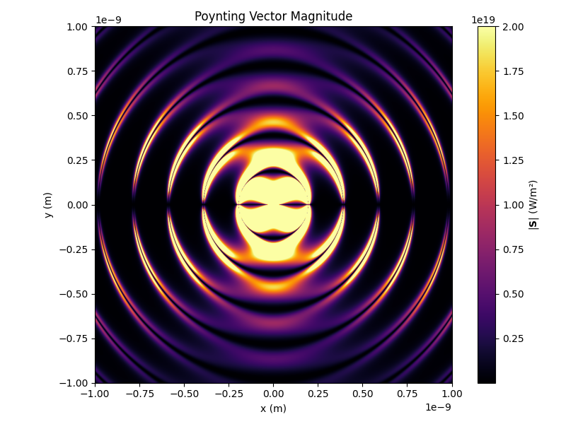
Poynting vector magnitude

The magnitude shows the energy flux density radiating from the oscillating dipole. The energy flows outward, strongest along directions perpendicular to the dipole axis.

fig, ax = plt.subplots(figsize=(8, 6))
im = ax.imshow(
    poynting_magnitude.T,
    origin="lower",
    cmap="inferno",
    extent=extent,
    vmax=2e19,
)
fig.colorbar(im, ax=ax, label=r"$|\mathbf{S}|$ (W/m²)")
ax.set_xlabel("x (m)")
ax.set_ylabel("y (m)")
ax.set_title("Poynting Vector Magnitude")
fig.tight_layout()
plt.show()