Quickstart#
Welcome to PyCharge! This quickstart provides a high-level introduction to the library’s core functionality and shows two minimal, reproducible examples you can run to get started.
PyCharge Workflows#
PyCharge supports two primary workflows:
Point-Charge Electromagnetics: Compute relativistically correct electromagnetic potentials and fields generated by point charges following predefined trajectories.
Self-Consistent N-Body Electrodynamics: Run time-domain simulations of multiple electromagnetic sources (e.g., dipoles) that interact through their self-generated fields.
This guide walks through both workflows with short examples.
Installation#
Install PyCharge with pip:
pip install pycharge
Note
For reliable numerical behavior, enable 64-bit floating-point precision in JAX. Add this line once near the top of your script or notebook:
jax.config.update("jax_enable_x64", True)
Part 1: Point-Charge Electromagnetics#
This section demonstrates computing electromagnetic potentials and fields produced by a point charge moving on a predefined trajectory.
1. Import the required libraries#
import jax
import jax.numpy as jnp
import matplotlib.pyplot as plt
from scipy.constants import c, e, m_e

from pycharge import Charge, dipole_source, potentials_and_fields, simulate

jax.config.update("jax_enable_x64", True)
2. Define a charge trajectory#
Provide a function that accepts a scalar time t and returns a position
tuple (x, y, z). PyCharge automatically differentiates this function to
obtain velocity and acceleration, so you only need to provide the position.
The example below creates a Charge that moves on a circle
in the x-y plane.
circular_radius = 1e-10
velocity = 0.9 * c
omega = velocity / circular_radius

def circular_position(t):
    x = circular_radius * jnp.cos(omega * t)
    y = circular_radius * jnp.sin(omega * t)
    z = 0.0
    return x, y, z

moving_charge = Charge(circular_position, e)
3. Build the potentials and fields function#
Use potentials_and_fields() with a list of charges to build a function that
computes the electromagnetic quantities (potentials and fields) at arbitrary observation points
and times. Wrap the returned function with jax.jit() to improve performance.
quantities_fn = potentials_and_fields([moving_charge])
jit_quantities_fn = jax.jit(quantities_fn)
4. Create an observation grid and evaluate#
Define a 2D observation plane (here: the x-y plane at z = 0 and
t = 0), build a mesh grid, and evaluate the JIT-compiled function on
that grid.
grid_size = 1000
xy_max = 5e-9
x_grid = jnp.linspace(-xy_max, xy_max, grid_size)
y_grid = jnp.linspace(-xy_max, xy_max, grid_size)
z_grid = jnp.array([0.0])
t_grid = jnp.array([0.0])

X, Y, Z, T = jnp.meshgrid(x_grid, y_grid, z_grid, t_grid, indexing="ij")

quantities = jit_quantities_fn(X, Y, Z, T)
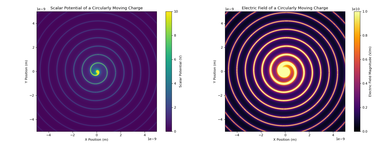
5. Visualize selected outputs#
The returned quantities is a NamedTuple containing
arrays for scalar and vector potentials and the electric and magnetic
fields. The example below plots the scalar potential and the magnitude of the electric field on
the observation plane.
scalar_potential = quantities.scalar
electric_field = quantities.electric
electric_field_magnitude = jnp.linalg.norm(electric_field, axis=-1)

fig, (ax1, ax2) = plt.subplots(1, 2, figsize=(16, 6))

im1 = ax1.imshow(
    scalar_potential.squeeze().T,
    extent=(x_grid.min(), x_grid.max(), y_grid.min(), y_grid.max()),
    origin="lower",
    cmap="viridis",
    vmax=10,
    vmin=0
)
fig.colorbar(im1, ax=ax1, label="Scalar Potential (V)")
ax1.set_xlabel("X Position (m)")
ax1.set_ylabel("Y Position (m)")
ax1.set_title("Scalar Potential of a Circularly Moving Charge")

im2 = ax2.imshow(
    electric_field_magnitude.squeeze().T,
    extent=(x_grid.min(), x_grid.max(), y_grid.min(), y_grid.max()),
    origin="lower",
    cmap="inferno",
    vmax=1e10,
    vmin=0,
)
fig.colorbar(im2, ax=ax2, label="Electric Field Magnitude (V/m)")
ax2.set_xlabel("X Position (m)")
ax2.set_ylabel("Y Position (m)")
ax2.set_title("Electric Field of a Circularly Moving Charge")

plt.tight_layout()
plt.show()
Part 2: Self-Consistent N-Body Electrodynamics#
PyCharge can simulate sources whose motion is governed by the electromagnetic fields they and
other sources produce. simulate() accepts a sequence of Source
objects and a discrete time grid, then integrates the coupled ODEs to produce time-evolving
source states.
1. Import the required libraries#
import jax
import jax.numpy as jnp
import matplotlib.pyplot as plt
from scipy.constants import e, m_e

from pycharge import dipole_source, simulate

jax.config.update("jax_enable_x64", True)
2. Create a dipole source#
Use dipole_source() to construct a Source that encapsulates
a dipole’s initial separation, physical parameters, and ODE.
dipole = dipole_source(
    d_0=[0.0, 0.0, 1e-9],
    omega_0=100e12 * 2 * jnp.pi,
    origin=[0.0, 0.0, 0.0],
    q=e,
    m=m_e,
)
3. Configure time steps and run the simulation#
Construct a time grid and run the simulation. For performance, JIT-compile
the function returned by simulate().
t_num = 40_000
dt = 1e-18
ts = jnp.arange(t_num) * dt

simulate_fn = jax.jit(simulate([dipole], ts))

source_states = simulate_fn()
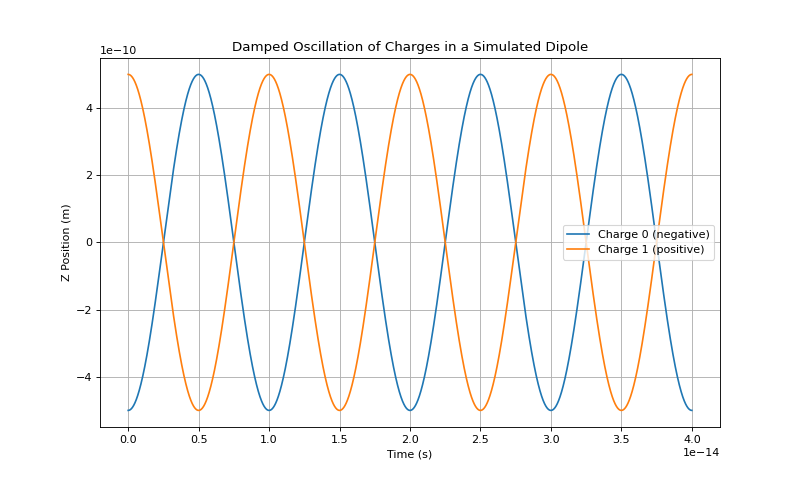
4. Analyze the simulation results#
source_states is a tuple of entries matching the input sources. Each
entry has shape (num_steps, num_charges, 2, 3) and stores positions and
velocities for every charge. The example below plots the z-coordinate of
the dipole’s charges over time.
dipole_state = source_states[0]

charge0_z_pos = dipole_state[:, 0, 0, 2]
charge1_z_pos = dipole_state[:, 1, 0, 2]

plt.figure(figsize=(10, 6))
plt.plot(ts, charge0_z_pos, label="Charge 0 (negative)")
plt.plot(ts, charge1_z_pos, label="Charge 1 (positive)")
plt.xlabel("Time (s)")
plt.ylabel("Z Position (m)")
plt.title("Damped Oscillation of Charges in a Simulated Dipole")
plt.legend()
plt.grid(True)
plt.show()